Benchmarks
Comparisons to other implementations of MPPI
| Parameter | Value |
|---|---|
| Dynamics parameters | |
| dt | 0.02s |
| wheel radius | 1.0m |
| wheel length | 1.0m |
| max velocity | 0.5m/s |
| min velocity | -0.35m/s |
| min rotation | -0.5rad/s |
| max rotation | 0.5rad/s |
| MPPI parameters | |
| $\lambda$ | 1.0 |
| control standard deviation | 0.2 |
| number of timesteps | 100 |
| Cost parameters | |
| Dist. to goal coeff. | 5 |
| Angular dist. to goal coeff. | 5 |
| Obstacle Cost | 20 |
| Map Width | 11m |
| Map Height | 11m |
| Map Resolution | 0.1m/cell |
In order to see the improvements our library can provide, we decided to compare against three other implementations of MPPI publicly available. The first comparison is with the MPPI implementation in AutoRally [1]. This implementation was the starting point of our new library, MPPI-Generic, and so we want to compare to see how well we can perform to our predecessor. The Autorally implementation is written in C++/CUDA, is compatible with ROS, features multiple dynamics models including linear basis functions, simple kinematics, and NN-based models focused on the Autorally hardware platform. There is only one Cost Function available but it does make use of CUDA textures for doing queries into an obstacle map. Additionally, it has been shown to run in real-time on hardware to great success [2], [3], [4]. However, the Autorally implementation is written mostly for use on the Autorally platform and as such, it has no general Cost Function, Dynamics, or Sampling Distribution APIs to extend. In order to use it for different problems such as flying a quadrotor, the MPPI implementation would need significant modification.
The next implementation we will compare against is Nav2’s MPPI. As of ROS Humble, there is a CPU implementation of MPPI in the ROS navigation stack [5]; for our testing, we utilized the version packaged for ROS 2 Iron. This CPU implementation [6] is written in C++ and looks to make heavy use of AVX instructions or vectorized instructions to improve performance. There is a small selection of dynamics models (Differential Drive, Ackermann, and Omni-directional) and cost functions that are focused around wheeled robots navigating through obstacle-laden environments. It allows users to implement new cost functions as critics through a plugin system and new dynamics models based off its MotionModel base class. This implementation will only become more widespread as ROS2 adoption continues to pick over the coming years, making it an essential benchmark. Unfortunately, it does have some drawbacks as it has no implementation of Tube-MPPI or RMPPI, and is only available in ROS2 Humble or newer. This means that it might not be usable on existing hardware platforms that are unable to upgrade their systems.
The last implementation of MPPI we will compare against is in TorchRL [7]. TorchRL is an open-source reinforcement learning Python library written by Meta AI, the developers of PyTorch itself. As such, it is widely trusted and available to researchers who are already familiar with PyTorch and Python. The TorchRL implementation works on both CPUs and GPUs and allows for custom dynamics and cost functions through the extension of base Environment class [8]. However, while it does have GPU support, it is limited to the functionality that PyTorch provides meaning that there is no option to use CUDA textures to improve map queries or any direct control of shared memory usage on the GPU. In addition, being written in Python makes it fairly legible and easy to extend but can come at the cost of performance when compared to C++ implementations.
In order to compare our library against these three implementations, we tried to recreate the same dynamics and cost function for each version of MPPI. We chose the Differential Drive dynamics model and some of the cost function components that already exist in the Nav2 implementation as the baseline. We used the goal position quadratic cost, goal angle quadratic cost, and the costmap-based obstacle cost components so that we could maintain a fairly simple cost function that allows us to show the capabilities of our library. We implemented these dynamics and cost functions in both CUDA and Python. The CUDA implementations were an extension of our base Dynamics and Cost Function APIs which allowed them to plug into our library easily. We decided to use the same code in the Autorally implementation as well which required some minor rewriting to account for different method names and state dimensions. The Python implementation was an extension of the TorchRL base Environment class, and was compiled using PyTorch’s JIT compiler in order to speed up performance when used in the TorchRL implementation. We used the same parameters for sampling, dynamics, cost function tuning, and MPPI hyperparameters across all implementations, summarized in Table 1.
| Parameter | Value |
|---|---|
| Dynamics thread block x dim | 64 |
| Dynamics thread block y dim | 4 |
| Cost thread block x dim | 64 |
| Cost thread block y dim | 1 |
For both Autorally and MPPI-Generic, there are some further performance enhancing options available such as block size choice. We ended up using the same block sizes for both Autorally and MPPI-Generic across all tests, shown in Table 2. As a result, the optimization times shown are not going to be the fastest possible performance that can be achieved on any given GPU but these tests should still serve as a useful benchmark to understand the average performance that can be achieved. We then ran each of the Autorally, MPPI-Generic, and Nav2 implementations $10,000$ times to produce optimal trajectories with $128$, $256$, $512$, $1024$, $2048$, $4096$, $6144$, $8192$, and $16,384$ samples; the TorchRL implementation was only run $1000$ times due to it being too slow to compute, even when using the GPU. This allowed us to produce more robust measurements of the computation times required as well as understand how well each implementation would scale as more computation was required. While our dynamics and cost functions currently chosen would not need up to $16,394$ samples, one might want to implement more complex dynamics or cost functions that could require a large number of samples to find the optimal solution. The comparisons were run across a variety of hardware including a Jetson Nano to see what bottlenecks each implementation might have. The Jetson Nano was unfortunately only able to run the MPPI-Generic and Autorally MPPI implementations as the last supported PyTorch version and the latest TorchRL libraries were incompatible, and the Nav2 implementation was unable to compile. GPUs tested ranged from a NVIDIA GTX 1050 Ti to a NVIDIA RTX 4090. Most tests were performed on an Intel 13900K which is one of the fastest available CPUs at the time of this writing in order to prevent the CPU being the bottleneck for the mostly GPU-based comparison; however, we did also run some tests on an AMD Ryzen 5 5600x to see the difference in performance on a lower-end CPU. % while the CPU options were either an Intel 13900K or an AMD Ryzen 5 5600x. The MPPI optimization times across all the hardware can be seen here and the code used to do these comparisons is available here.
Results
 Fig. 1: Optimization times for all MPPI implementations on a hardware system with a RTX 4090 and an Intel 13900K over a variety of number of samples.
It can be seen that the Nav2 CPU implementation grows linearly as the number of samples increase while GPU implementations grow more slowly.
Fig. 1: Optimization times for all MPPI implementations on a hardware system with a RTX 4090 and an Intel 13900K over a variety of number of samples.
It can be seen that the Nav2 CPU implementation grows linearly as the number of samples increase while GPU implementations grow more slowly.
Going over all of the collected data would take too much room for this paper so we shall instead try to pull out interesting highlights to discuss. First, we can look at the results on the most powerful system tested, using an Intel i9-13900K and an NVIDIA RTX 4090 in Fig. 1. As the number of samples increase, the CPU-bound Nav2 method increases in optimization times in a linear fashion immediately. Every other method uses the GPU which can provide headroom to increase the number of samples as the GPU is not fully utilized at small sample sizes. We also see that as we hit $16,384$ samples, the AutoRally implementation starts to have lower optimization times than MPPI-Generic. We will see this trend continue in Fig. 2.
 Fig. 2: Optimization times for all MPPI implementations on a hardware system with a GTX 1050 Ti and an Intel 13900K over a variety of number of samples. It can be seen that MPPI-Generic and AutoRally on this older hardware does eventually start to scale linearly with the number of samples but does so at a much lower rate with our library compared to Nav2 or Pytorch.
When looking at older and lower-end NVIDIA hardware such as the GTX 1050 Ti, we still see that our library still performs well compared to other implementations as seen in Fig. 2. Only when the number of samples is at $128$ does the Nav2 implementation on an Intel 13900k match the performance of the AutoRally implementation on this older GPU. However, we can see that Nav2 implementation again outperforms the TorchRL implementation until we hit $16,384$ samples. MPPI-Generic is still more performant at these lower number of samples and eventually we see it scales linearly as we get to thousands of samples. The TorchRL implementation also finally starts to show some GPU bottle-necking as we start to see optimization times increasing as we reach over $6144$ samples. We can also see that there is a moment where the MPPI-Generic library optimization time grows to be larger than the AutoRally implementation. That occurs when we switch from using the split kernels to the combined kernel discussed here. The AutoRally implementation uses a combined kernel as well but has fewer synchronization points on the GPU due to strictly requiring forward Euler integration for the dynamics. At the small hit to performance in the combined kernel, our library allows for many more features, such as multi-threaded cost functions, use of shared memory in the cost function, and implementation of more computationally-heavy integration methods such as Runge-Kutta or backward Euler integration. And while we see a hit to performance when using the combined kernel compared to AutoRally, we still see that the split kernel is faster for up to $2048$ samples.
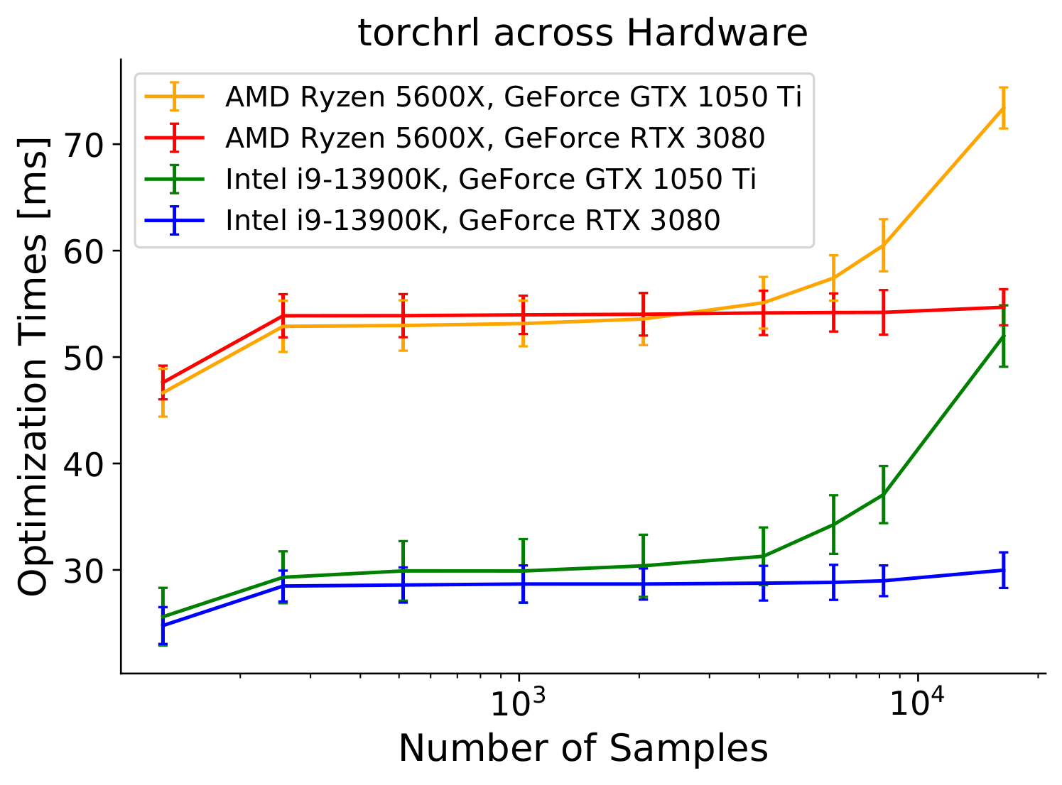 Fig. 3: Optimization times for the TorchRL implementation across different CPUs and GPUs. We see that TorchRL computation times are more dependent on the CPU as the RTX 3080 with an AMD 5600X ends up slower than a GTX 1050 Ti with an Intel 13900k.
The TorchRL implementation is notably performing quite poorly in Figs. 1 and 2 with runtimes being around $28$ ms no matter the number of samples. Looking at TorchRL-specific results in Fig. 3, we can see that the TorchRL implementation seems to be heavily CPU-bound. A low-end GPU (1050 Ti) combined with a high-end CPU (Intel 13900K) can achieve better optimization times than a low-end CPU (AMD 5600X) combined with a high-end GPU (RTX 3080).
We also conducted tests on a 2019 Jetson Nano to show that even on relatively low-power and older systems, our library can still be used. As the latest version of CUDA supporting the Jetson Nano is 10.2 and the OS is Ubuntu 18.04, both the pytorch and Nav2 MPPI implementations were not compatible. As such, we only have results comparing our MPPI-Generic implementation to the AutoRally implementation in Fig. 4. Here, we can see that the AutoRally implementation starts having faster compute times around $512$ samples. Again, this is due to our library switching to the combined kernel which will be slower. However, our library on a Jetson Nano at $2048$ samples has a roughly equivalent computation time to that of $2048$ samples of the Nav2 implementation on the Intel 13900K processor, showing that our GPU parallelization can allow for real time optimization even on portable systems.
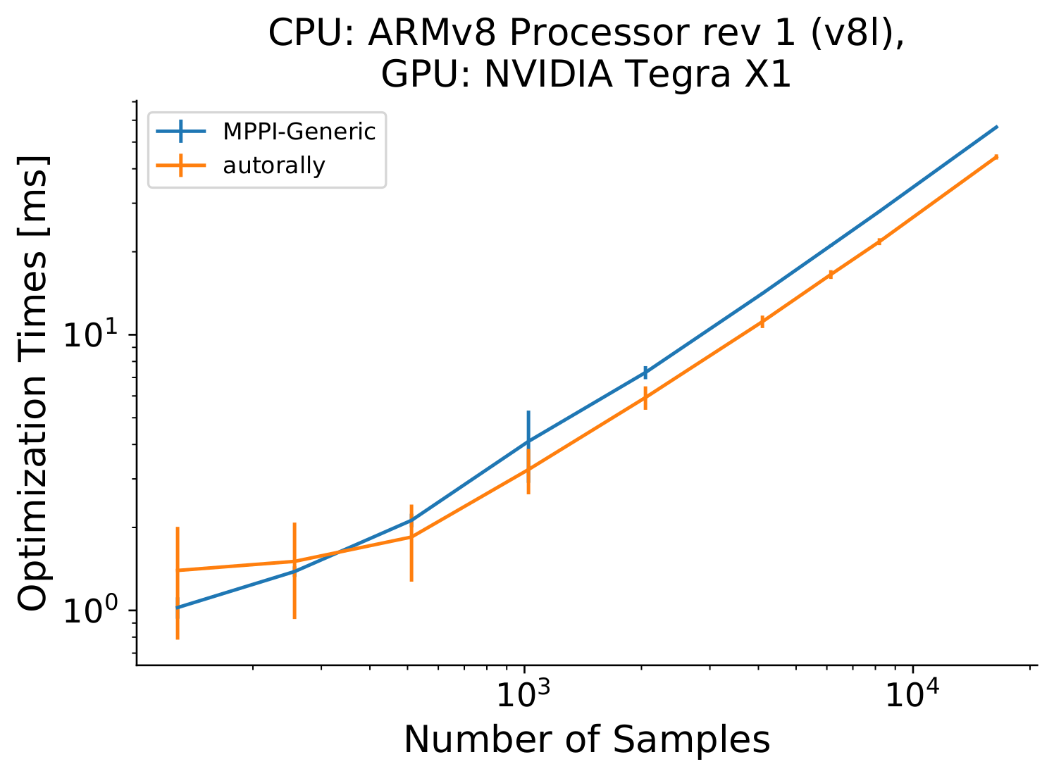 Fig. 4: Optimization times for MPPI implementations on a Jetson Nano over a variety of number of samples. It can be seen that MPPI-Generic and AutoRally on this low-power hardware can still achieve sub 10 ms optimization times for even 2048 samples. The AutoRally implementation quickly surpasses our implementation in optimization times.
In addition, we can really see the benefits of our library as we increase the computation time of the cost function. At this point, the pytorch and Nav2 implementations have been shown to be slow in comparison to the other implementations and are thus dropped from this cost complexity comparison.
float computeStateCost(...) {
    float cost = 1.0;
    for (int i = 0; i < NUM_COSINES; i++) {
        cost = cos(cost);
    }
    cost *= 0.0;
    // Continue to regular cost function
    ...
}
Listing 1: Computation time inflation code added to the cost function. We add a configurable amount of calls to cos() as this is a computationally heavy function to run.
We can artificially inflate the computation time of the cost function with Lst. 1 to judge how well the implementations scale to more complex cost functions. In Fig 5, we see how increasing the computation time of the cost function scales for both implementations over the same hardware and for the same number of samples.
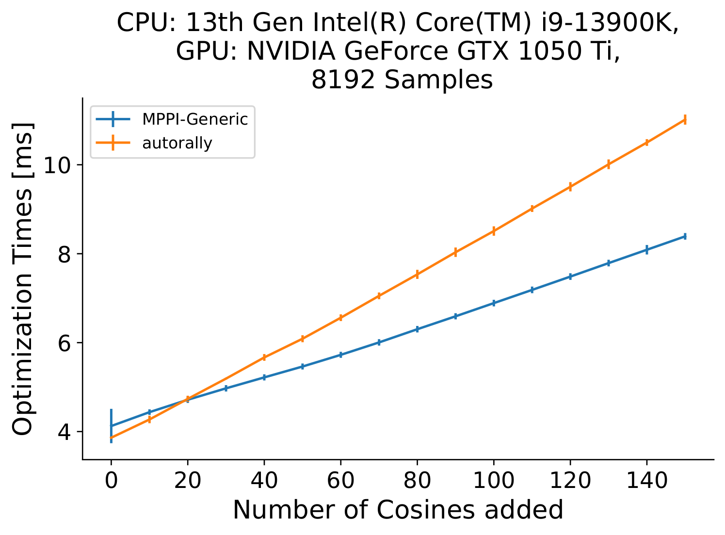 Fig. 5: Optimization Times for MPPI-Generic and AutoRally implementations as the computation time of the cost function increases.
Using an Intel 13900K, NVIDIA GTX 1050 Ti, and 8192 samples, we can see that the our library implementation starts to outperform the AutoRally implementation when 20+ sequential cosine operations are added to the cost function.
Fig. 5: Optimization Times for MPPI-Generic and AutoRally implementations as the computation time of the cost function increases.
Using an Intel 13900K, NVIDIA GTX 1050 Ti, and 8192 samples, we can see that the our library implementation starts to outperform the AutoRally implementation when 20+ sequential cosine operations are added to the cost function.
Comparisons to sampling-efficent algorithms
While we have shown that our implementation of MPPI can have faster computation times and a lot of flexibility in where it can be applied, there remains a question of what is the balance point between number of samples and real time performance. Ideally, we would like to sample all possible paths to calculate the optimal control trajectory but this is computationally infeasible. While our work has decreased the computation time for sampling which in turn allows more samples in the same computation time, other works have tried to reduce the amount of samples needed to evaluate the optimal control trajectory. In [9], the authors introduce a generalization of MPC algorithms called Dynamic Mirror Descent Model Predictive Control (DMD-MPC) defined by the choice of shaping function, $S(\cdot)$, Sampling Distribution $\pi_\theta$, and Bregman Divergence $D_\Psi(\cdot, \cdot)$ which determines how close the new optimal control trajectory should remain to the previous. Using the exponential function, Gaussian sampling, and the KL Divergence, they derive a slight modification to the MPPI update law that introduces a step size parameter $\gamma_t \geq 0$:
\[\begin{align} u_{t}^{k+1} = \PP{1 - \gamma_t} u_{t}^k + \gamma_t \frac{\Expectation[V \sim \pi_\theta]{\Shape\PP{\J\PP{X,V}}v_t}}{\Expectation[V \sim \pi_\theta]{\Shape\PP{\J\PP{X,V}}}}, \end{align}\]where $v_t$ is the control value at time $t$ from the sampled control sequence $V$, and $\J$ is the Cost Function. In their results, they showed that when using a low number of samples, the addition of a step size can help improve performance. However, once the number of samples increases beyond a certain point, the optimal step size ends up being $1.0$ which is equivalent to the original MPPI update law. Having this option is useful in cases where you have a low computational budget. What we would like to show is that as long as you have a NVIDIA GPU from the last decade, you can have enough computational budget to just use more samples instead of needing to tune a step size.
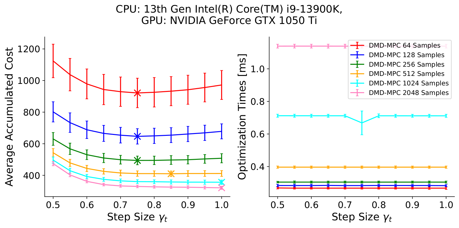 Fig. 6: Average Accumulated Costs (left) and Optimization Times (right) with error bars signifying one standard deviation for a variety of step sizes and number of samples for DMD-MPC.
$\times$ indicates the step size that achieves the lowest cost for a given number of samples.
This was run on a 2D double integrator dynamics with a cost shown in \eqref{eq:double_integrator_circle_cost}.
This system was run for 1000 timesteps to get the accumulated cost and this was repeated 1000 times to get the standard deviation bars shown.
When using a low number of samples, a lower DMD-MPC step size provides the lowest costs.
However, as the number of samples increase, the best step size choice becomes $\gamma_t = 1.0$ which is equivalent to the normal MPPI update law.
For our library, increasing the number of samples to the point where the step size is no longer useful is still able to be run at over 800 Hz on the NVIDIA GTX 1050 Ti.
Fig. 6: Average Accumulated Costs (left) and Optimization Times (right) with error bars signifying one standard deviation for a variety of step sizes and number of samples for DMD-MPC.
$\times$ indicates the step size that achieves the lowest cost for a given number of samples.
This was run on a 2D double integrator dynamics with a cost shown in \eqref{eq:double_integrator_circle_cost}.
This system was run for 1000 timesteps to get the accumulated cost and this was repeated 1000 times to get the standard deviation bars shown.
When using a low number of samples, a lower DMD-MPC step size provides the lowest costs.
However, as the number of samples increase, the best step size choice becomes $\gamma_t = 1.0$ which is equivalent to the normal MPPI update law.
For our library, increasing the number of samples to the point where the step size is no longer useful is still able to be run at over 800 Hz on the NVIDIA GTX 1050 Ti.
Looking at Fig. 6, we ran a 2D double integrator system with state $[x,y,v_x,v_y]$ and control $[a_x, a_y]$ with the cost shown in \eqref{eq:double_integrator_circle_cost}:
\[\begin{align} J &= 1000 \PP{\mathbb{I}_{\left\{\PP{x^2+y^2} \leq 1.875^2\right\}} + \mathbb{I}_{\left\{\PP{x^2+y^2} \geq 2.125^2\right\}}} + 2\abs{2 - \sqrt{v_x^2 + v_y^2}} + 2\abs{4 - \PP{xv_y - yv_x}}. \label{eq:double_integrator_circle_cost} \end{align}\]This cost function heavily penalizes the system from leaving a circle of radius $2$m with width $0.125$m but gives no cost inside the track width, has an $L_1$ cost on speed to maintain $2$m/s, and has an $L_1$ cost on the angular momentum being close to $4$m^2/s. This all combines to encourage the system to move around the circle allowing some small deviation from the center line in a clockwise manner. This system was simulated for 1000 timesteps and the cost was accumulated over that period. This simulation was run 1000 times to ensure consistent cost evaluations. We see that as the number of samples increase, the optimal step size (marked with a x) increases to $1.0$. In addition, the computation time increase for using a number of samples where the step size is irrelevant is minimal (an increase of about $0.04$ ms).
References
[1] B. Goldfain, P. Drews, G. Williams, and J. Gibson, AutoRally, Georgia Tech AutoRally Organization. [Online]. Available: https://github.com/AutoRally/autorally
[2] B. Goldfain, P. Drews, C. You, M. Barulic, O. Velev, P. Tsiotras, and J. M. Rehg, “Autorally: An open platform for aggressive autonomous driving,” IEEE Control Systems Magazine, vol. 39, no. 1, pp. 26–55, 2019
[3] G. Williams, P. Drews, B. Goldfain, J. M. Rehg, and E. A. Theodorou, “Aggressive Driving with Model Predictive Path Integral Control,” in 2016 IEEE International Conference on Robotics and Automation (ICRA). IEEE, 2016, pp. 1433–1440. [Online]. Available: https://ieeexplore.ieee.org/document/7487277/
[4] G. Williams, P. Drews, B. Goldfain, J. M. Rehg, and E. A. Theodorou, “Information-Theoretic Model Predictive Control: Theory and Applications to Autonomous Driving,” IEEE Transactions on Robotics, vol. 34, no. 6, pp. 1603-1622, 2018. [Online]. Available: https://ieeexplore.ieee.org/document/8558663
[5] S. Macenski, T. Moore, D. Lu, A. Merzlyakov, and M. Ferguson, “From the Desks of ROS Maintainers: A Survey of Modern & Capable Mobile Robotics Algorithms in the Robot Operating System 2,” Robotics and Autonomous Systems, vol. 168, p. 104493, 2023. [Online]. Available: https://www.sciencedirect.com/science/article/pii/S092188902300132X
[6] A. Budyakov and S. Macenski, “ROS2 Model Predictive Path Integral Controller,” Open Navigation, Version 1.2.4. [Online]. Available: https://github.com/ros-planning/navigation2/tree/iron/nav2_mppi_controller
[7] A. Bou, M. Bettini, S. Dittert, V. Kumar, S. Sodhani, X. Yang, G. D. Fabritiis, and V. Moens, “TorchRL: A data-driven decision-making library for PyTorch,” in The Twelfth International Conference on Learning Representations, Jan. 2024. [Online]. Available: https://openreview.net/forum?id=QxItoEAVMb
[8] torchrl contributors, “mppi.py - pytorch/rl,” Meta, 2023. Version 0.2.1. [Online]. Available: https://github.com/pytorch/rl/blob/main/torchrl/modules/planners/mppi.py
[9] N. Wagener, C.-A. Cheng, J. Sacks, and B. Boots, “An Online Learning Approach to Model Predictive Control,” in Proceedings of Robotics: Science and Systems, Freiburg im Breisgau, Germany, Jun. 2019. [Online]. Available: http://arxiv.org/abs/1902.08967