Performance Implementation

We now will go over some of the performance-specific implementation details we make use of in MPPI-Generic. First, we will give a brief introduction to GPU hardware and terminology followed by general GPU performance tricks. We will then dive into computational optimizations that are specific to the tasks our library is used to solve.

GPU Parallelization Overview

The GPU is a highly parallelizable hardware device that performs operations a bit differently from a CPU. The lowest level of computation in CUDA is a warp, which consists of 32 threads doing the same operation at every clock step. These warps are grouped together to produce thread blocks. The individual warps in the thread block are not guaranteed to be at the same place in the code at any given time and sometimes it can actually be more efficient to allow them to differ. The threads in a thread block all have access a form of a local cache called shared memory. Like any memory shared between multiple threads on the CPU, proper mutual exclusion needs to be implemented to avoid race conditions. Threads in a block can be given indices in 3 axes, x, y, and z, which we use to denote different types of parallelization within the library. Thread blocks can themselves be grouped into grids and are also organized into x, y, and z axes. This is useful for large parallel operations that cannot fit within a single thread block and also do not need to use shared memory between every thread. The GPU code is compiled into kernels, which can then be provided arbitrary grid and block dimensions at runtime.

It is important to briefly understand the hierarchy of memory before discussing how to improve GPU performance. At the highest level, we have global memory which is generally measured in GBs and very slow to access data from. Next, we have an L2 cache in the size of MBs which can speed up access to frequently-used global data. Then we have the L1 cache, shared memory, and CUDA texture caches. The L1 cache and shared memory are actually the same memory on hardware and are generally several KBs in size; they are just separated by programmers explicitly using shared memory and the GPU automatically filling the L1 cache. The CUDA texture cache is a fast read-only memory used for CUDA textures which are 2D or 3D representations of data such as a map.

General GPU speedups

When looking into writing more performant code, there are some general tricks that we have leveraged throughout our code library. The first is the use of CUDA streams [1]. By default, every call to the GPU blocks the CPU code from moving ahead. CUDA streams allow for the asynchronous scheduling of tasks on the GPU while the CPU performs other work in the meantime. We use CUDA streams throughout in order to schedule memory transfers between the CPU and GPU as well as kernel calls and have different streams for controller optimal control computation and visualization.

The next big tip is minimizing global memory accesses. Global memory reading or writing can be a large bottleneck in computation time and for our library, it can take up more time than the actual computations we want to do on the GPU. The first step recommended is to move everything you can from global memory to shared memory [2]. We also make use of Curiously Recurring Template Patterns (CRTPs) [3] as our choice of polymorphism on the GPU as to avoid the need of constructing and reading from a virtual method table which would need to be stored in global memory. In addition, we utilize vectorized memory [4] accessing where possible. Looking at the GPU instruction set, CUDA provides instructions to read and write in 32, 64, and 128 bit chunks in a single instruction. This means that it is possible to load up to four 32-bit floats in a single instruction. Using these concepts, we greatly reduce the number of calls to global memory and consequently increase the speed at which our computations can run.

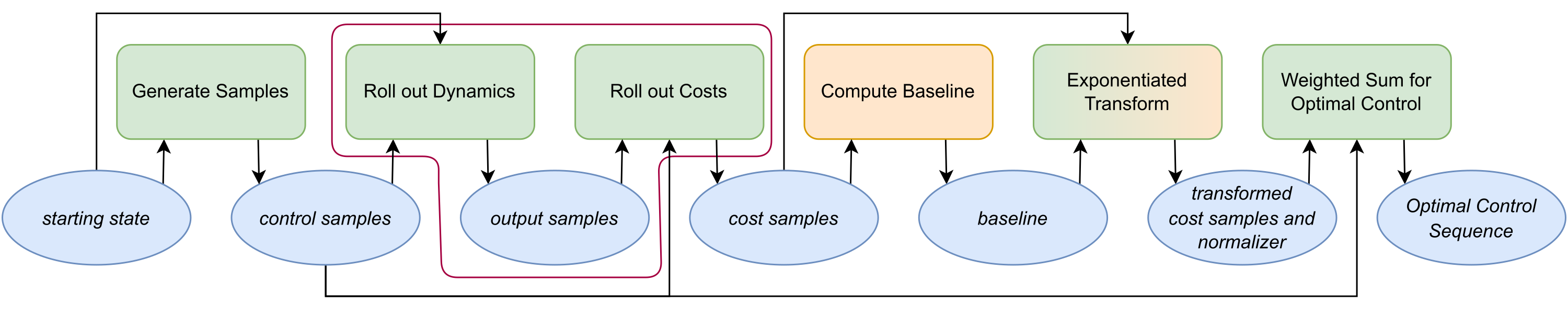Fig. 1: Diagram of the execution flow of computeControl(). The blue ellipses indicate variables, the green rectangles are GPU methods, and the orange rectangles are CPU methods. The selection in purple is a single GPU kernel when using the combined kernel and separated out when using split kernels. Most of the code is run on the GPU but we have found that some operations such as finding the baseline run faster on the CPU.

Library-Specific Performance Optimizations

So far, we have discussed optimizations that can be done for any CUDA program. However, there are further optimizations to be had in choosing how to parallelize specific components of our library. In Fig. 1, we have the general steps taken every time we want to compute a new optimal control sequence in MPPI. These same steps are also taken in Tube-MPPI and RMPPI though they have to be done for both the nominal and real systems.

One major performance consideration is how to parallelize the Dynamics and Cost Function calculations. We have found that, depending on the circumstances and the number of samples used in MPPI, different parallelization techniques make more sense. One way would be to run the Dynamics and Cost Function in a combined kernel on the GPU while another would be to run them in separate kernels. We discuss the description as well as the pros and cons of each parallelization technique below.

Split Kernels

We start by taking the initial state and control samples and run them through the Dynamics kernel. This kernel uses all three axes of thread parallelization for different components. First, the x dimension of the block and the grid are used to indicate which sample we are on as threadIdx.x + blockDim.x * blockIdx.x. As every sample should go through the exact same computations, using the x axis allows us to ensure that each warp is aligned. Next, the z axis is used to indicate which system is being run; for MPPI, there is only one system but Tube-MPPI and RMPPI use two systems, nominal and real. Finally, the y dimension is used to parallelize within the dynamics function As dynamics are rarely doing the same derivative computation for every state, this additional parallelization within the dynamics, shown in Lst. 1, can lead to better performance rather than sequentially going through each calculation. In the Dynamics kernel, we then run a for loop over time for each sample in which we get the current control sample, runs it through the Dynamic’s step() method, and save out the resulting output to global memory.

int tdy = threadIdx.y;
switch(tdy) {
  case S_INDEX(X):
    xdot[tdy] = u[C_INDEX(VEL)]*cos(x[S_INDEX(YAW)]);
    break;
  case S_INDEX(Y):
    xdot[tdy] = u[C_INDEX(VEL)]*sin(x[S_INDEX(YAW)]);
    break;
  case S_INDEX(YAW):
    xdot[tdy] = u[C_INDEX(YAW_DOT)];
    break;
}

Listing 1: GPU code for the Unicycle Dynamics. This code parallelizes using the thread y dimension to do each state derivative calculation in a different thread

Now, we could have also run the Cost Function inside the previous kernel but we instead separate it out into its own kernel. The reason for that is that while the Dynamics must be sequential over time, the cost function does not need to be. To achieve this, we move the sample index up to the grid level and use the block’s x axes for time instead. The Cost kernel gets the control and output corresponding to the current time in its computeRunningCost() or terminalCost() methods, adds the cost up across time for each sample, and saves out the resulting overall cost for each sample. A problem that might arise with this implementation is that we might become limited in the number of timesteps we could optimize over due there being a limit of 1024 threads in a single thread block. In order to address this, we calculate the max number of iterations over the thread x dimension required to achieve the desired number of timesteps and conduct a for loop over that iteration count. So for example, if we had 500 as the desired number of timesteps and block x size of 128, we would do four iterations in our for loop to get the total horizon cost. These choices brings the time to do the cost calculation to much closer to that of a single timestep instead of having to wait for sequential iterations of the cost if it was paired with the Dynamics kernel.

Combined Kernel

The Combined Kernel runs the Dynamics and Cost Function methods together in a single kernel. This works by getting the initial state and control samples, applying the Dynamics’ step() to get the next state and output, and running that output through the Cost Functions’ computeCost() to get the cost at that time. This basic interaction is then done in a for loop over the time horizon to get the the entire state trajectory as well as the cost of the entire sample. We parallelize this over three axes. First, the x and z dimensions of the block and grid are used to indicate which sample and system we are on as described above in the Split Kernel’s Dynamics section. Finally, the y dimension is used to parallelize within the Dynamics and Cost Functions’ methods.

Choosing between the Split and Combined Kernels

There are some trade-offs between the two kernel options that can affect the overall computation time. By combining the Dynamics and Cost Function calculations together, we can keep the intermediate outputs in shared memory and don’t need to save them out to global memory. However, we are forced to run the Cost Function sequentially in time. Splitting the Dynamics and Cost Function into separate kernels allows them each to use more shared memory for their internal calculations with the requirement of global memory usage to save out the sampled output trajectories. The Combined Kernel uses less global memory but requires more shared memory usage in a single kernel as it must contain both the Dynamics and Cost Functions’ shared memory requiremens. As the number of samples grow, the number of reads and writes of outputs to global memory also grows. This can eventually take more time to do than the savings we get from running the Cost Function in parallel across time, even when using vectorized memory reads and writes.

In order to address these trade-offs, we have implemented both kernel approaches in our library and automatically choose the most appropriate kernel at Controller construction. The automatic kernel selection is done by running both the combined and split kernels multiple times and then choosing the fastest option. As the combined kernel potentially uses more shared memory than the split kernel, we also check to see if the amount of shared memory used is below the GPU’s shared memory hardware limit; if it is not, we default to the split kernel approach. We also allow the user to overwrite the automatic kernel selection through the use of the setKernelChoice() method.

Weight Transform and Update Rule Kernels

Once the costs of each sample trajectory is calculated, we then bring these costs back to the CPU in order to find the baseline, ρ. The baseline is calculated by finding the minimum cost of all the sample trajectories; it is subtracted out during the exponentiation stage as it has empirically led to better optimization performance. When the number of samples is only in the thousands, we have found that the copy to the CPU to do the baseline search is faster than attempting to do the search on the GPU.

References

[1] M. Harris, “How to Overlap Data Transfers in CUDA C/C++,” Dec. 2012. [Online]. Available: https://developer.nvidia.com/blog/how-overlap-data-transfers-cuda-cc/

[2] M. Harris, “Using Shared Memory in CUDA C/C++,” Jan. 2013. [Online]. Available: https://developer.nvidia.com/blog/using-shared-memory-cuda-cc/

[3] J. O. Coplien, Curiously recurring template patterns, C++ Report, vol. 7, no. 2, pp. 24-27, 1995

[4] J. Luitjens, “CUDA Pro Tip: Increase Performance with Vectorized Memory Access,”” Dec. 2013. [Online]. Available: https://developer.nvidia.com/blog/cuda-pro-tip-increase-performance-with-vectorized-memory-access/